fABBA

An efficient symbolic aggregate approximation for temporal data 🐬

The ABBA methods perform a fast and accurate symbolic approximation for temporal data. fABBA is a Python library for the efficient implementation of ABBA methods, which is based on a polygonal chain approximation of the time series followed by an aggregation of the polygonal pieces into groups.

The fABBA library supports different ABBA methods, for example, ABBA and fABBA (in contrast to the software fABBA), whose aggregation process is sped up by sorting the polygonal pieces and exploiting early termination conditions. However, the approximation of fABBA is less accurate than ABBA. In contrast to the ABBA method [S. Elsworth and S. Güttel, Data Mining and Knowledge Discovery, 34:1175-1200, 2020], fABBA avoids repeated within-cluster-sum-of-squares computations which reduces its computational complexity significantly. Furthermore, fABBA is fully tolerance-driven and does not require the number of time series symbols to be specified by the user.

🚀 Install

fABBA supports Linux, Windows, and MacOS operating system.

fABBA has the following essential dependencies for its functionality:

* cython (>= 0.29.7)
* numpy (>= 1.19.5)
* scipy (>=1.2.1)
* requests
* scikit-learn (>=0.17.1)
* threadpoolctl (>= 2.0.0)
* matplotlib

To ensure successful Cython compiling, please update your NumPy to the latest version>= 1.22.0.

To install the current release via PIP use:

pip install fabba

Download this repository:

git clone https://github.com/nla-group/fABBA.git

It also supports conda-forge install:

To install this package via conda-forge, run the following: conda install -c conda-forge fabba

🏁 Examples

⭐ Compress and reconstruct a time series

The following example approximately transforms a time series into a symbolic string representation (transform) and then converts the string back into a numerical format (inverse_transform). fABBA essentially requires two parameters tol and alpha. The tolerance tol determines how closely the polygonal chain approximation follows the original time series. The parameter alpha controls how similar time series pieces need to be in order to be represented by the same symbol. A smaller tol means that more polygonal pieces are used and the polygonal chain approximation is more accurate; but on the other hand, it will increase the length of the string representation. A smaller alpha typically results in a larger number of symbols.

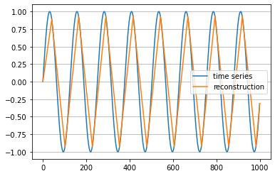
The choice of parameters depends on the application, but in practice, one often just wants the polygonal chain to mimic the key features in time series and not to approximate any noise. In this example the time series is a sine wave and the chosen parameters result in the symbolic representation BbAaAaAaAaAaAaAaC. Note how the periodicity in the time series is nicely reflected in repetitions in its string representation.

import numpy as np
import matplotlib.pyplot as plt
from fABBA import fABBA

ts = [np.sin(0.05*i) for i in range(1000)]  # original time series
fabba = fABBA(tol=0.1, alpha=0.1, sorting='2-norm', scl=1, verbose=0)

string = fabba.fit_transform(ts)            # string representation of the time series
print(string)                               # prints aBbCbCbCbCbCbCbCA

inverse_ts = fabba.inverse_transform(string, ts[0]) # numerical time series reconstruction

Plot the time series and its polygonal chain reconstruction:

plt.plot(ts, label='time series')
plt.plot(inverse_ts, label='reconstruction')
plt.legend()
plt.grid(True, axis='y')
plt.show()

To play fABBA further with real datasets, we recommend users start with UCI Repository and UCR Archive.

⭐ Adaptive polygonal chain approximation

Instead of using fit_transform which combines the polygonal chain approximation of the time series and the symbolic conversion into one, both steps of fABBA can be performed independently. Here’s how to obtain the compression pieces and reconstruct time series by inversely transforming the pieces:

import numpy as np
from fABBA import compress
from fABBA import inverse_compress
ts = [np.sin(0.05*i) for i in range(1000)]
pieces = compress(ts, tol=0.1)               # pieces is a list of the polygonal chain pieces
inverse_ts = inverse_compress(pieces, ts[0]) # reconstruct polygonal chain from pieces

Similarly, the digitization can be implemented after compression step as below:

from fABBA import digitize
from fABBA import inverse_digitize
string, parameters = digitize(pieces, alpha=0.1, sorting='2-norm', scl=1) # compression of the polygon
print(''.join(string))                                 # prints aBbCbCbCbCbCbCbCA

inverse_pieces = inverse_digitize(string, parameters)
inverse_ts = inverse_compress(inverse_pieces, ts[0])   # numerical time series reconstruction

⭐ Alternative ABBA approach

We also provide other clustering based ABBA methods, it is easy to use with the support of scikit-learn tools. The user guidance is as follows

import numpy as np
from sklearn.cluster import KMeans
from fABBA import ABBAbase

ts = [np.sin(0.05*i) for i in range(1000)]         # original time series
#  specifies 5 symbols using kmeans clustering
kmeans = KMeans(n_clusters=5, random_state=0, init='k-means++', n_init='auto', verbose=0)     
abba = ABBAbase(tol=0.1, scl=1, clustering=kmeans)
string = abba.fit_transform(ts)                    # string representation of the time series
print(string)                                      # prints BbAaAaAaAaAaAaAaC
inverse_ts = abba.inverse_transform(string)        # reconstruction

fABBA is an extensive package, which includes all ABBA variants, you can use the original ABBA method via

from fABBA import ABBA
abba = ABBA(tol=0.1, scl=1, k=5, verbose=0)
string = abba.fit_transform(ts)
print(string)
inverse_ts = abba.inverse_transform(string, ts[0])

⭐ For multiple time series data transform

Load JABBA package and data:

from fABBA import JABBA
from fABBA import loadData
train, test = loadData()

Built in JABBA provide parameter of init for the specification of ABBA methods, if set agg, then it will automatically turn to fABBA method, and if set it to k-means, it will turn to ABBA method automatically. Use JABBA object to fit and symbolize the train set via API fit_transform, and reconstruct the time series from the symbolic representation simply by

jabba = JABBA(tol=0.0005, init='agg', verbose=1)
symbols = jabba.fit_transform(train) 
reconst = jabba.inverse_transform(symbols)

Note: function loadData() is a lightweight API for time series dataset loading, which only supports part of data in UEA or UCR Archive, please refer to the document for full use detail. JABBA is used to process multiple time series as well as multivariate time series, so the input should be ensured to be 2-dimensional, for example, when loading the UCI dataset, e.g., Beef, use symbols = jabba.fit_transform(train) , when loading UEA dataset, e.g., BasicMotions, use symbols = jabba.fit_transform(train[0]) . For details, we refer to (https://www.cs.ucr.edu/~eamonn/time_series_data_2018/).

For the out-of-sample data, use the function transform to symbolize the test time series, and reconstruct the symbolization via function inverse_transform, the code illustration is as follows:

test_symbols, start_set = jabba.transform(test) # if UEA time series is used, simply use instead jabba.transform(test[0])
test_reconst = jabba.inverse_transform(test_symbols, start_set)

⭐ Image compression

The following example shows how to apply fABBA to image data.

import matplotlib.pyplot as plt
from fABBA.load_datasets import load_images
from fABBA import image_compress
from fABBA import image_decompress
from fABBA import fABBA
from cv2 import resize
img_samples = load_images() # load test images
img = resize(img_samples[0], (100, 100)) # select the first image for test

fabba = fABBA(tol=0.1, alpha=0.01, sorting='2-norm', scl=1, verbose=1)
string = image_compress(fabba, img)
inverse_img = image_decompress(fabba, string)

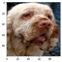
Plot the original image:

plt.imshow(img)
plt.show()

Plot the reconstructed image:

plt.imshow(inverse_img)
plt.show()

🎨 Experiments

The folder "exp" contains all code required to reproduce the experiments in the manuscript "An efficient aggregation method for the symbolic representation of temporal data".

Some of the experiments also require the UCR Archive 2018 datasets which can be downloaded from UCR Time Series Classification Archive.

There are a number of dependencies listed below. Most of these modules, except perhaps the final ones, are part of any standard Python installation. We list them for completeness:

os, csv, time, pickle, numpy, warnings, matplotlib, math, collections, copy, sklearn, pandas, tqdm, tslearn

Please ensure that these modules are available before running the codes. A numpy version newer than 1.19.0 and less than 1.20 is required.

It is necessary to compile the Cython files in the experiments folder (though this is already compiled in the main module, the experiments code is separated). To compile the Cython extension in "src" use:

cd exp/src
python3 setup.py build_ext --inplace

or

cd exp/src
python setup.py build_ext --inplace

💌 Others

We also provide C++ implementation for fABBA in the repository cabba, it would be nice to give a shot!

Run example:

git clone https://github.com/nla-group/fABBA.git
cd fABBA/cpp
g++ -o test runtime.cpp
./test

📎 Citation

If you use fABBA in a scientific publication, we would appreciate your citing:

@article{10.1145/3532622,
author = {Chen, Xinye and G\"{u}ttel, Stefan},
title = {An Efficient Aggregation Method for the Symbolic Representation of Temporal Data},
year = {2023},
publisher = {ACM},
volume = {17},
number = {1},
doi = {10.1145/3532622},
journal = {ACM Transactions on Knowledge Discovery from Data},
numpages = {22},
}

If you have any questions, please be free to reach us!

📝 License

This project is licensed under the terms of the .